


3.1 人和马分类
准备工作
从网络上下载资源
!wget --no-check-certificate \
    https://storage.googleapis.com/laurencemoroney-blog.appspot.com/horse-or-human.zip \
    -O /tmp/horse-or-human.zip
使用python代码将使用OS库来调用文件系统,并使用zipfile库来解压数据。
import os
import zipfile

local_zip = '/tmp/horse-or-human.zip'
zip_ref = zipfile.ZipFile(local_zip, 'r')
zip_ref.extractall('/tmp/horse-or-human')
zip_ref.close()Zip文件的内容会被解压到目录/tmp/horse-or-human,而该目录下又分别包含horses和humans子目录。
简而言之:训练集就是用来告诉神经网络模型 "这就是马的样子"、"这就是人的样子 "等数据。
这里需要注意的是,我们并没有明确地将图像标注为马或人。如果还记得之前的手写数字例子,它的训练数据已经标注了 "这是一个1","这是一个7 "等等。 稍后,我们使用一个叫做ImageGenerator的类--用它从子目录中读取图像,并根据子目录的名称自动给图像贴上标签。所以,会有一个 "训练 "目录,其中包含一个 "马匹 "目录和一个 "人类 "目录。ImageGenerator将为你适当地标注图片,从而减少一个编码步骤。(不仅编程上更方便,而且可以避免一次性把所有训练数据载入内存,而导致内存不够等问题。)
让我们分别定义这些目录。
# Directory with our training horse pictures
train_horse_dir = os.path.join('/tmp/horse-or-human/horses')

# Directory with our training human pictures
train_human_dir = os.path.join('/tmp/horse-or-human/humans')
现在,让我们看看 "马 "和 "人 "训练目录中的文件名是什么样的。
train_horse_names = os.listdir(train_horse_dir)
print(train_horse_names[:10])

train_human_names = os.listdir(train_human_dir)
print(train_human_names[:10])

['horse39-1.png', 'horse47-6.png', 'horse12-1.png', 'horse23-7.png', 'horse11-0.png', 'horse50-8.png', 'horse38-5.png', 'horse42-3.png', 'horse29-5.png', 'horse36-6.png']

['human09-00.png', 'human09-14.png', 'human11-11.png', 'human04-14.png', 'human14-14.png', 'human07-03.png', 'human06-04.png', 'human09-29.png', 'human08-03.png', 'human14-16.png']
我们来看看目录中马和人的图片总数。
print('total training horse images:', len(os.listdir(train_horse_dir)))
print('total training human images:', len(os.listdir(train_human_dir)))

## total training horse images: 500
## total training human images: 527
现在我们来看看几张图片,以便对它们的样子有个直观感受。首先,配置matplot参数.(可选)
%matplotlib inline

import matplotlib.pyplot as plt
import matplotlib.image as mpimg

# Parameters for our graph; we'll output images in a 4x4 configuration
nrows = 4
ncols = 4

# Index for iterating over images
pic_index = 0
接下来,显示一批8张马和8张人的图片。每次重新运行单元格,都会看到一个新的批次即另外8张马和8张人.(可选)
# Set up matplotlib fig, and size it to fit 4x4 pics
fig = plt.gcf()
fig.set_size_inches(ncols * 4, nrows * 4)

pic_index += 8
next_horse_pix = [os.path.join(train_horse_dir, fname)
                for fname in train_horse_names[pic_index-8:pic_index]]
next_human_pix = [os.path.join(train_human_dir, fname)
                for fname in train_human_names[pic_index-8:pic_index]]

for i, img_path in enumerate(next_horse_pix+next_human_pix):
  # Set up subplot; subplot indices start at 1
  sp = plt.subplot(nrows, ncols, i + 1)
  sp.axis('Off') # Don't show axes (or gridlines)

  img = mpimg.imread(img_path)
  plt.imshow(img)

plt.show()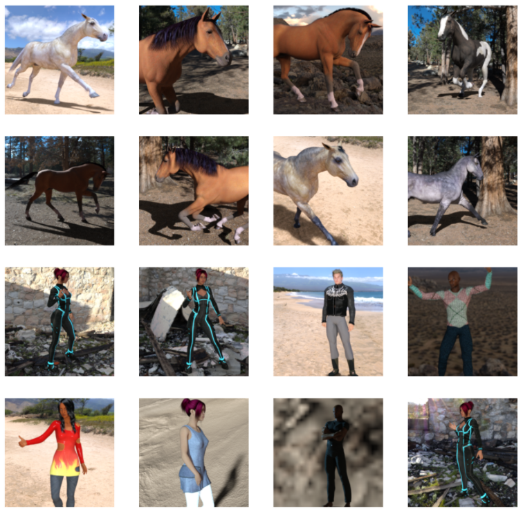
定义模型
# 第一步是导入 tensorflow.
import tensorflow as tf

# 然后,像前面的例子一样添加卷积层,并将最终结果扁平化,以输送到全连接的层去。
# 最后我们添加全连接层。
# 需要注意的是,由于我们面对的是一个两类分类问题,即二类分类问题,所以我们会用sigmoid激活函数作为模型的最后一层,这样我们网络的输出将是一个介于0和1之间的有理数,即当前图像是1类(而不是0类)的概率。

model = tf.keras.models.Sequential([
    # Note the input shape is the desired size of the image 300x300 with 3 bytes color
    # This is the first convolution
    tf.keras.layers.Conv2D(16, (3,3), activation='relu', input_shape=(150, 150, 3)),
    tf.keras.layers.MaxPooling2D(2, 2),
    # The second convolution
    tf.keras.layers.Conv2D(32, (3,3), activation='relu'),
    tf.keras.layers.MaxPooling2D(2,2),
    # The third convolution
    tf.keras.layers.Conv2D(64, (3,3), activation='relu'),
    tf.keras.layers.MaxPooling2D(2,2),
    # The fourth convolution
    tf.keras.layers.Conv2D(64, (3,3), activation='relu'),
    tf.keras.layers.MaxPooling2D(2,2),
    # The fifth convolution
    tf.keras.layers.Conv2D(64, (3,3), activation='relu'),
    tf.keras.layers.MaxPooling2D(2,2),
    # Flatten the results to feed into a DNN
    tf.keras.layers.Flatten(),
    # 512 neuron hidden layer
    tf.keras.layers.Dense(512, activation='relu'),
    # Only 1 output neuron. It will contain a value from 0-1 where 0 for 1 class ('horses') and 1 for the other ('humans')
    tf.keras.layers.Dense(1, activation='sigmoid')
调用model.summary()方法打印出神经元网络模型的结构信息,方便学习。
model.summary()Model: "sequential"
_________________________________________________________________
Layer (type) Output Shape Param #
=================================================================
conv2d (Conv2D) (None, 148, 148, 16) 448
_________________________________________________________________
max_pooling2d (MaxPooling2D) (None, 74, 74, 16) 0
_________________________________________________________________
conv2d_1 (Conv2D) (None, 72, 72, 32) 4640
_________________________________________________________________
max_pooling2d_1 (MaxPooling2 (None, 36, 36, 32) 0
_________________________________________________________________
conv2d_2 (Conv2D) (None, 34, 34, 64) 18496
_________________________________________________________________
max_pooling2d_2 (MaxPooling2 (None, 17, 17, 64) 0
_________________________________________________________________
conv2d_3 (Conv2D) (None, 15, 15, 64) 36928
_________________________________________________________________
max_pooling2d_3 (MaxPooling2 (None, 7, 7, 64) 0
_________________________________________________________________
conv2d_4 (Conv2D) (None, 5, 5, 64) 36928
_________________________________________________________________
max_pooling2d_4 (MaxPooling2 (None, 2, 2, 64) 0
_________________________________________________________________
flatten (Flatten) (None, 256) 0
_________________________________________________________________
dense (Dense) (None, 512) 131584
_________________________________________________________________
dense_1 (Dense) (None, 1) 513
=================================================================
Total params: 229,537
Trainable params: 229,537
Non-trainable params: 0"输出形状 "一栏显示了特征图尺寸在每个层中是如何演变的。卷积层由于边框关系而使特征图的尺寸减小了一些,而每个池化层则将输出尺寸减半。
接下来,我们将配置模型训练的参数。我们将用 "binary_crossentropy(二元交叉熵)"衡量损失,因为这是一个二元分类问题,最终的激活函数是一个sigmoid。我们将使用rmsprop作为优化器,学习率为0.001。在训练过程中,我们将希望监控分类精度。
from tensorflow.keras.optimizers import RMSprop

model.compile(loss='binary_crossentropy',
              optimizer=RMSprop(lr=0.001),
              metrics=['acc'])
数据预处理(此步操作可提前)
让我们设置训练数据生成器(ImageDataGenerator),它将读取源文件夹中的图片,将它们转换为float32多维数组,并将图像数据(连同它们的标签)反馈给神经元网络。总共需要两个生成器,有用于产生训练图像,一个用于产生验证图像。生成器将产生一批大小为300x300的图像及其标签(0或1)。
前面的课中我们已经知道如何对训练数据做归一化,进入神经网络的数据通常应该以某种方式进行归一化,以使其更容易被网络处理。在这个例子中,我们将通过将像素值归一化到[0, 1]范围内(最初所有的值都在[0, 255]范围内)来对图像进行预处理。
from tensorflow.keras.preprocessing.image import ImageDataGenerator

# All images will be rescaled by 1./255
train_datagen = ImageDataGenerator(rescale=1/255)

# Flow training images in batches of 128 using train_datagen generator
train_generator = train_datagen.flow_from_directory(
        '/tmp/horse-or-human/',  # This is the source directory for training images
        target_size=(150, 150),  # All images will be resized to 150x150
        batch_size=32, #128
        # Since we use binary_crossentropy loss, we need binary labels
        class_mode='binary')

## Found 1027 images belonging to 2 classes.
开始训练
让我们训练15个epochs--这可能需要几分钟的时间完成运行。
请注意每次训练后的数值。
损失和准确率是训练进展的重要指标。模型对训练数据的类别进行预测,然后根据已知标签进行评估,计算准确率。准确率是指正确预测的比例。
history = model.fit(
      train_generator,
      steps_per_epoch=8,
      epochs=15,
      verbose=1)
Epoch 1/15
8/8 [==============================] - 2s 267ms/step - loss: 0.6917 - acc: 0.5117
Epoch 2/15
8/8 [==============================] - 2s 285ms/step - loss: 0.5690 - acc: 0.7227
Epoch 3/15
8/8 [==============================] - 2s 278ms/step - loss: 0.3585 - acc: 0.8477
Epoch 4/15
8/8 [==============================] - 2s 236ms/step - loss: 0.3443 - acc: 0.8899
Epoch 5/15
8/8 [==============================] - 2s 283ms/step - loss: 0.2400 - acc: 0.9219
Epoch 6/15
8/8 [==============================] - 2s 277ms/step - loss: 0.2330 - acc: 0.9219
Epoch 7/15
8/8 [==============================] - 2s 264ms/step - loss: 0.1396 - acc: 0.9492
Epoch 8/15
8/8 [==============================] - 2s 274ms/step - loss: 0.2055 - acc: 0.9258
Epoch 9/15
8/8 [==============================] - 2s 268ms/step - loss: 0.0746 - acc: 0.9736
Epoch 10/15
8/8 [==============================] - 2s 251ms/step - loss: 0.4834 - acc: 0.8899
Epoch 11/15
8/8 [==============================] - 2s 263ms/step - loss: 0.1158 - acc: 0.9688
Epoch 12/15
8/8 [==============================] - 2s 268ms/step - loss: 0.0967 - acc: 0.9609
Epoch 13/15
8/8 [==============================] - 2s 281ms/step - loss: 0.0534 - acc: 0.9883
Epoch 14/15
8/8 [==============================] - 2s 252ms/step - loss: 0.0880 - acc: 0.9559
Epoch 15/15
8/8 [==============================] - 2s 255ms/step - loss: 0.0892 - acc: 0.9648用模型进行预测
接下来,看看使用模型进行实际预测。这段代码将允许你从文件系统中选择1个或多个文件,然后它将上传它们,并通过模型判断给出图像是马还是人。
import numpy as np
from google.colab import files
from tensorflow.keras.preprocessing import image

uploaded = files.upload()

for fn in uploaded.keys():

  # predicting images
  path = '/content/' + fn
  img = image.load_img(path, target_size=(300, 300))
  x = image.img_to_array(img)
  x = np.expand_dims(x, axis=0)

  images = np.vstack([x])
  classes = model.predict(images, batch_size=10)
  print(classes[0])
  if classes[0]>0.5:
    print(fn + " is a human")
  else:
    print(fn + " is a horse")
关于自动调参
构造神经元网络模型时,一定会考虑需要几个卷积层?过滤器应该几个?全连接层需要几个神经元?
最先想到的肯定是手动修改那些参数,然后观察训练的效果(损失和准确度),从而判断参数的设置是否合理。但是那样很繁琐,因为参数组合会有很多,训练时间很长。再进一步,可以手动编写一些循环,通过遍历来搜索合适的参数。但是最好利用专门的框架来搜索参数,不太容易出错,效果也比前两种方法更好。
Kerastuner就是一个可以自动搜索模型训练参数的库。它的基本思路是在需要调整参数的地方插入一个特殊的对象(可指定参数范围),然后调用类似训练那样的search方法即可。
接下来首先准备训练数据和需要加载的库。
import os
from tensorflow.keras.preprocessing.image import ImageDataGenerator
from tensorflow.keras.optimizers import RMSprop
train_datagen = ImageDataGenerator(rescale=1/255)
validation_datagen = ImageDataGenerator(rescale=1/255)
train_generator = train_datagen.flow_from_directory('/tmp/horse-or-human/',
        target_size=(150, 150),batch_size=32,class_mode='binary')
validation_generator = validation_datagen.flow_from_directory('/tmp/validation-horse-or-human/',
        target_size=(150, 150), batch_size=32,class_mode='binary')
from kerastuner.tuners import Hyperband
from kerastuner.engine.hyperparameters import HyperParameters
import tensorflow as tf
接着创建HyperParameters对象,然后在模型中插入Choice、Int等调参用的对象。
hp=HyperParameters()
def build_model(hp):
    model = tf.keras.models.Sequential()
    model.add(tf.keras.layers.Conv2D(hp.Choice('num_filters_top_layer',values=[16,64],default=16), (3,3),
                                     activation='relu', input_shape=(150, 150, 3)))
    model.add(tf.keras.layers.MaxPooling2D(2, 2))
    for i in range(hp.Int("num_conv_layers",1,3)):
        model.add(tf.keras.layers.Conv2D(hp.Choice(f'num_filters_layer{i}',values=[16,64],default=16), (3,3), activation='relu'))
        model.add(tf.keras.layers.MaxPooling2D(2,2))
    model.add(tf.keras.layers.Flatten())
    model.add(tf.keras.layers.Dense(hp.Int("hidden_units",128,512,step=32), activation='relu'))
    model.add(tf.keras.layers.Dense(1, activation='sigmoid'))
    model.compile(loss='binary_crossentropy',optimizer=RMSprop(lr=0.001),metrics=['acc'])
    return model
然后创建Hyperband对象,这是Kerastuner支持的四种方法的其中一种,其优点是能较四童话第查找参数。具体资料可以到Kerastuner的网站获取。
最后调用search方法。
tuner=Hyperband(
    build_model,
    objective='val_acc',
    max_epochs=10,
    directory='horse_human_params',
    hyperparameters=hp,
    project_name='my_horse_human_project'
)
tuner.search(train_generator,epochs=10,validation_data=validation_generator)
搜索到最优参数后,可以通过下面的程序,用tuner对象提取最优参数构建神经元网络模型。并调用summary方法观察优化后的网络结构。
best_hps=tuner.get_best_hyperparameters(1)[0]
print(best_hps.values)
model=tuner.hypermodel.build(best_hps)
model.summary()
释放资源
运行以下单元格可以终止内核并释放内存资源。当计算资源不够时需要进行释放。
import os, signal
os.kill(os.getpid(), signal.SIGKILL)
Comments NOTHING